Introduction
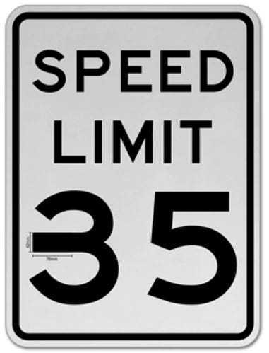
To you and me, that sign says 35 mph. A self-driving car might read it as 85. Researchers have shown exactly that: tiny, barely visible changes to a speed limit sign can make a Tesla's vision system misclassify it. That's an evasion attack: small perturbations that push a machine learning model to the wrong answer while looking fine to humans.
ML models are everywhere now: facial recognition, fraud detection, malware scanners, autonomous systems. They're powerful and brittle. Understanding how adversaries think is central to red teaming and offensive security research. This post walks through how adversaries trick them. We'll cover four attack families:
- White box attacks: full access to the model's internals
- Black box attacks: only the final decision is visible
- Gray box attacks: probability scores or partial outputs
- Transfer-based attacks: craft on one model, deploy on another
Same goal in each case: find inputs the model misclassifies. The tactics differ by how much the attacker can see.
Background: How Models Learn (and Where They're Fragile)
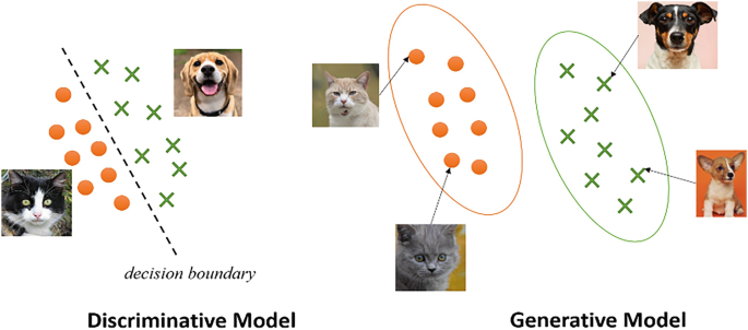
A model is a function that maps inputs to outputs, trained on data to classify images, predict values, or the like. Classifiers put things in buckets (cat vs. dog); regressors predict numbers (e.g. house price). Training adjusts the model's parameters to minimize error. The result is a decision boundary: the surface that separates one predicted class from another.
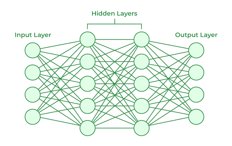
Optimization techniques like gradient descent move the parameters toward a minimum of the loss. In high dimensions, though, those decision boundaries aren't solid walls: they're thin, and small changes to the input can push it across. Adversarial attacks target exactly those fragile regions.
Adversarial Examples
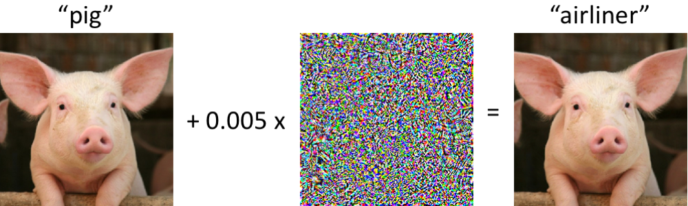
Inputs that look virtually identical to humans can make a model output the wrong class. Small, crafted perturbations exploit the fragile decision boundaries we just talked about.
How you attack depends on what you can observe. Two dimensions matter: how much access you have to the model, and whether you want any wrong answer or a specific one.
Levels of Model Access
Attack strategies are primarily defined by how much an attacker knows about the model:
- White-Box Attacks: The attacker has full access to the model's architecture, weights, and gradients.
- Gray-Box Attacks: The attacker has partial access, often seeing output probabilities but not internal mechanics.
- Black-Box Attacks: The attacker only knows the final decision (e.g., "yes" or "no") without insight into how it was reached.
Targeted vs. Non-Targeted Attacks
Beyond the level of access, the intent of the attack further differentiates these strategies:
- Targeted Attacks: The attacker wants a specific incorrect output (e.g., making a "stop" sign appear as a "speed limit" sign).
- Non-Targeted Attacks: The goal is simply to cause an incorrect classification, regardless of the specific output.
Detailed Exploration of Evasion Attack Techniques
White-Box Attacks
With full access to the model (architecture, weights, gradients), an attacker can craft very effective adversarial examples. The 2015 Goodfellow et al. paper is still the right place to start.
Fast Gradient Sign Method (FGSM)
FGSM uses the gradient of the loss with respect to the input: take its sign, scale by ε, and add it to the input in one step. Single-step, fast, and surprisingly effective. The classic demo is a panda image perturbed until the model labels it a gibbon with high confidence, with changes almost invisible to a human.
FGSM Implementation in PyTorch
import torch
import torch.nn.functional as F

def fgsm_attack(model, image, label, epsilon):
"""Generates an adversarial example using FGSM."""
image.requires_grad = True # Enable gradient tracking for the input
output = model(image) # Forward pass
loss = F.nll_loss(output, label) # Compute loss
model.zero_grad() # Reset gradients
loss.backward() # Compute gradients
perturbation = epsilon * image.grad.sign() # Compute adversarial perturbation
adversarial_image = image + perturbation # Apply perturbation
adversarial_image = torch.clamp(adversarial_image, 0, 1) # Ensure valid pixel values
return adversarial_image
Projected Gradient Descent (PGD) Attack
PGD is FGSM done iteratively: small gradient steps, projected back into an ε-ball around the original input. In practice we reach for PGD more than FGSM when we have gradients: it finds stronger adversarial examples and often bypasses defenses that only consider single-step attacks.
PGD Implementation in PyTorch
import torch.optim as optim

def pgd_attack(model, image, label, epsilon, alpha, num_iter):
"""Generates an adversarial example using PGD."""
perturbed_image = image.clone().detach().requires_grad_(True)

    for _ in range(num_iter):
        output = model(perturbed_image)
        loss = F.nll_loss(output, label)
        model.zero_grad()
        loss.backward()
        perturbation = alpha * perturbed_image.grad.sign()  # Small step in gradient direction
        perturbed_image = perturbed_image + perturbation  # Apply perturbation
        perturbed_image = torch.clamp(perturbed_image, image - epsilon, image + epsilon)  # Project back
        perturbed_image = torch.clamp(perturbed_image, 0, 1)  # Keep within valid pixel range
        perturbed_image = perturbed_image.detach().requires_grad_(True)  # Reset for next iteration

    return perturbed_image
Carlini & Wagner (C&W) Attack
C&W frames the problem as optimization: find the smallest perturbation that forces misclassification. It uses gradient descent (e.g. Adam) on the input and a confidence term to tune how aggressive the perturbation is. Result: very small, often hard-to-detect changes. It's been used to bypass commercial malware detectors: adjust a few features of a malicious file and the classifier flips.
C&W Attack Implementation in PyTorch
import torch.optim as optim

def cw_attack(model, image, label, confidence=0, lr=0.01, max_iter=1000):
"""Generates an adversarial example using the Carlini & Wagner attack."""
perturbed_image = image.clone().detach().requires_grad_(True)
optimizer = optim.Adam([perturbed_image], lr=lr)

    for _ in range(max_iter):
        output = model(perturbed_image)
        loss = -F.nll_loss(output, label) + confidence  # Minimize perturbation while ensuring misclassification
        model.zero_grad()
        optimizer.zero_grad()
        loss.backward()
        optimizer.step()  # Update the perturbation

    return perturbed_image.detach()
Jacobian-Based Saliency Map Attack (JSMA)
JSMA perturbs only the most influential pixels. It builds a saliency map from the Jacobian, then flips a small set of pixels until the model's prediction changes. Fewer changes than a full gradient attack, and you can target a specific wrong class.
JSMA Implementation in PyTorch
import torch

def jsma_attack(model, image, target_label, num_features):
"""Generates an adversarial example using the Jacobian-based Saliency Map Attack (JSMA)."""
perturbed_image = image.clone().detach().requires_grad_(True)

    for _ in range(num_features):
        output = model(perturbed_image)
        loss = -F.nll_loss(output, target_label)
        model.zero_grad()
        loss.backward()
        saliency = perturbed_image.grad.abs()
        max_saliency = torch.argmax(saliency)
        perturbed_image.view(-1)[max_saliency] += 0.1  # Slightly modify the most influential pixel

    return perturbed_image.detach()
Defenses that only consider single-step attacks (e.g. FGSM) are insufficient; PGD and C&W routinely get through. If an attacker has gradient access, assume they can produce adversarial examples: adversarial training and certified defenses are the direction that actually holds up.
Gray-Box Attacks
When you don't have gradients but you do have output probabilities (or soft labels), you can still approximate a direction to perturb. ZOO does it with finite differences: probe the model with small input changes, estimate the gradient from the output shifts, then update. NES uses a different idea: sample random perturbations, keep the ones that hurt the true class, and iterate. Square Attack restricts changes to small square patches in the image, which cuts down the number of queries. All three have been shown to work against real systems: cloud vision APIs (e.g. Google Cloud Vision), fraud detectors (transactions tweaked until classified legitimate), and robust image classifiers that use JPEG compression or smoothing. Localized or query-efficient attacks can still get through.
Black-Box Attacks
When the only thing you get from the model is the final label (no probabilities, no gradients), you're in the black-box setting. Query-based and transfer-based methods still work.
The HopSkipJump Attack
HopSkipJump is built for label-only access. You start from a misclassified input and nudge it along the decision boundary with minimal queries, refining until you have a small adversarial perturbation. No gradient estimates, just boundary probing.
HopSkipJump in PyTorch
import torch

def hopskipjump_attack(model, image, target_label, num_iter=50, step_size=0.01):
"""Black-box attack using decision boundary exploration."""
perturbed_image = image.clone()

    for _ in range(num_iter):
        # Generate random perturbation direction
        direction = torch.randn_like(image).sign()

        # Test the perturbation
        test_image = perturbed_image + step_size * direction
        if model(test_image).argmax() == target_label:
            perturbed_image = test_image  # Keep the adversarial example

    return perturbed_image.detach()
HopSkipJump and similar ideas have been used against cloud ML APIs (e.g. Google Cloud Vision) and fraud detection: repeated queries with small changes until the model flips.
The Boundary Attack
Boundary Attack starts from a wrong classification (e.g. random noise the model labels as something) and walks it toward the clean input while keeping the label wrong. You end up with a minimal adversarial example. No gradients or scores required.
Boundary Attack in PyTorch
import torch

def boundary_attack(model, image, target_class, step_size=0.01, num_iter=100):
"""Boundary Attack: Starts with an adversarial example and refines it."""
perturbed_image = torch.randn_like(image) # Start with random noise

    for _ in range(num_iter):
        perturbed_image = perturbed_image + step_size * (image - perturbed_image)
        output = model(perturbed_image)
        if output.argmax() == target_class:
            break  # Stop when the target misclassification is achieved

    return perturbed_image.detach()
The famous Tesla case fits here: researchers put small stickers on a 35 mph sign and got the car's vision system to read 85 mph. Fully black-box: no access to the model. Physical adversarial examples are a real risk for autonomous vehicles and similar systems.
The One-Pixel Attack
Change one pixel (or a handful). A genetic-algorithm-style search finds which pixel and what value cause misclassification. Surprisingly effective and very hard to spot. It's been used to break image classifiers (panda→gibbon), fool facial recognition, and defeat CAPTCHAs.
One-Pixel Attack in PyTorch
import torch
import random

def one_pixel_attack(model, image, label, num_iterations=100):
"""One-Pixel Attack: Modifies a single pixel to fool the classifier."""
perturbed_image = image.clone()

    for _ in range(num_iterations):
        x, y = random.randint(0, image.shape[2] - 1), random.randint(0, image.shape[3] - 1)
        perturbed_image[:, :, x, y] = torch.rand(1)  # Change one pixel

        if model(perturbed_image).argmax() != label:
            break  # Stop when misclassification occurs

    return perturbed_image.detach()
Transfer-Based Attacks
Adversarial examples often transfer: an input that fools one model frequently fools another. So you can train a substitute model (on data labeled by the target, or on a similar dataset), craft adversarial examples on the substitute with white-box methods, and fire them at the real target without ever touching its internals.
The Substitute Model Attack
Papernot et al. (2017): query the target for labels, train a surrogate on those labels, then run FGSM or similar on the surrogate. The resulting adversarial examples often transfer to the target with high success rates (e.g. 80%+).
Code Example: Training a Substitute Model in PyTorch
import torch
import torch.nn as nn
import torch.optim as optim

def train_substitute_model(target_model, train_loader, num_epochs=5):
"""Trains a substitute model by querying the target model for labels."""
substitute_model = nn.Sequential(
nn.Conv2d(3, 16, kernel_size=3, stride=1, padding=1),
nn.ReLU(),
nn.Flatten(),
nn.Linear(16 * 32 * 32, 10) # Assuming CIFAR-10
)

    optimizer = optim.Adam(substitute_model.parameters(), lr=0.001)
    loss_fn = nn.CrossEntropyLoss()

    for epoch in range(num_epochs):
        for images, _ in train_loader:
            labels = target_model(images).argmax(dim=1)  # Querying the target model for labels
            optimizer.zero_grad()
            outputs = substitute_model(images)
            loss = loss_fn(outputs, labels)
            loss.backward()
            optimizer.step()

    return substitute_model  # Trained to imitate the target model
Momentum Iterative FGSM (MI-FGSM)
Early transfer attacks overfitted to the substitute. Dong et al. (2018) added momentum to the gradient updates so the perturbations generalize better across models. Standard choice when you care about transferability.
MI-FGSM in PyTorch
import torch

def mi_fgsm_attack(model, image, label, epsilon, alpha, num_iter, decay_factor=1.0):
"""Momentum Iterative FGSM (MI-FGSM) attack for transferability."""
perturbed_image = image.clone().detach().requires_grad_(True)
momentum = torch.zeros_like(image)

    for _ in range(num_iter):
        output = model(perturbed_image)
        loss = torch.nn.functional.cross_entropy(output, label)

        model.zero_grad()
        loss.backward()

        grad = perturbed_image.grad.data
        momentum = decay_factor * momentum + grad / torch.norm(grad, p=1)  # Apply momentum
        perturbation = alpha * momentum.sign()  # Compute adversarial perturbation

        perturbed_image = perturbed_image + perturbation
        perturbed_image = torch.clamp(perturbed_image, image - epsilon, image + epsilon)  # Keep within bounds
        perturbed_image = perturbed_image.detach().requires_grad_(True)  # Reset for next step

    return perturbed_image
Ensemble Attacks
Craft adversarial examples against several substitute models at once; the combined perturbation often transfers better to an unseen target because it hits shared decision boundaries. Higher success rates in practice.
Ensemble Attack in PyTorch
def ensemble_attack(models, image, label, epsilon):
"""Generates an adversarial example that transfers across multiple models."""
perturbed_image = image.clone().detach().requires_grad_(True)

    for model in models:  # Loop through multiple substitute models
        output = model(perturbed_image)
        loss = torch.nn.functional.cross_entropy(output, label)

        model.zero_grad()
        loss.backward()

        perturbation = epsilon * perturbed_image.grad.sign()
        perturbed_image = perturbed_image + perturbation
        perturbed_image = torch.clamp(perturbed_image, 0, 1)  # Ensure valid pixel values

    return perturbed_image.detach()
Adversarial patches take this into the physical world: a pattern on a T-shirt (2020 work used MI-FGSM and ensembles) that makes person detectors fail, and the same patch transferred across multiple detectors. So you don't need to query the target at all: train surrogates, craft on them, and the examples often still work. Input filtering and defensive distillation usually aren't enough against good transfer attacks.
Conclusion
Assume your model is white-box to an attacker who can query it: that's the safe assumption for deployment. If they only get labels, transfer and query-based attacks still work. Defenses that help: adversarial training, certified robustness where feasible, and input preprocessing that's validated against the same attack class you care about. For a practical next step, run PGD on your own models and see how many queries it takes to break them; then treat that as a baseline for what an adversary might do. If your application relies on ML models, application penetration testing should include adversarial input testing as part of the scope.
Written by
Founder of PlatformSecurity and veteran security expert with over a decade of experience in offensive security. Recognized penetration testing specialist who has uncovered critical vulnerabilities in Fortune 500 companies, cloud infrastructure, and enterprise applications. Expert in red team operations, cloud security, and vulnerability research with a track record of responsible disclosures and high-impact security findings.